A high level introduction to Cache Memories
Why study Caches?
Let me first introduce a very simple problem of adding a scalar to each element of a 2D matrix. There are two ways in which I can do this:
- Access elements row wise
function rowAccess(A::AbstractMatrix) for i in 1:size(A)[1] for j in 1:size(A)[2] A[i,j] = A[i,j]+1 end end return A end - Access elements column wise
  function colAccess(A::AbstractMatrix)
      for i in 1:size(A)[1]
          for j in 1:size(A)[2]
              A[j,i] = A[j,i]+1
          end
      end
      return A
  end
I’ll be using Julia Programming language but feel free to follow along with any programming language.
When I run both of these independently (supplying \(5000\times5000\) matrix A) and benchmark it, I observe that the function rowAccess takes 160.2 ms to run while colAccess finishes in 16.4 ms!!
@btime _ = colAccess(A);
16.400 ms (0 allocations: 0 bytes)
@btime _ = rowAccess(A);
160.207 ms (0 allocations: 0 bytes)
Both of these results can be explained easily after a good understanding of Caches, hence it’s imperative that every programmer must understand how memories work in modern computers. In this blog post, I’ll be explaining the basic concepts related to Memory Heirarchy, so that you can start writing cache friendly code and avoid mistakes such the one in function rowAccess.
If you try to do the same thing in C/C++, you’ll notice that row access runs faster than column access. Don’t worry, this is normal and by the end of this post you’ll have the answer to this as well.
Introduction
For most of the basic programming tasks, a simple model of a computer system is assumed in which CPU executes instructions and a memory system holds data/instructions for the CPU. This memory is assumed to be a linear array of bytes, where each memory location can be accessed in constant amount of time.
In practice, a memory system is a hierarchy of storage devices with different capacities, costs and access times.
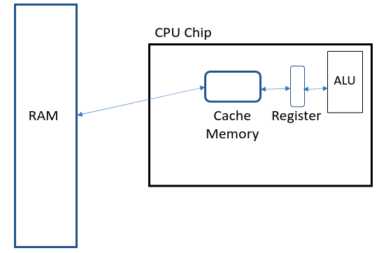
From the figure above you can see different types of storage devices:
- Registers: Very small in size (few KBs), very fast access times, very expensive.
- Caches: Small in size (100s of KBs to few MBs), fast access times, expensive.
- RAM: Large in size (few GBs), moderate access times, moderate cost.
Access time is the time required to move data to the ALU for processing.
Let’s now see in detail how these memories work by going through the code example line by line.
I’ll be discussing the details in a very abstract manner where I’ll not be diving into the bit-wise representation of arrays. So just remember that the way data is stores in RAM or cache is a bit more complicated than what I’ll be discussing. However I’ll cover these minute details in some other blog post.
Random Access Memory (RAM)
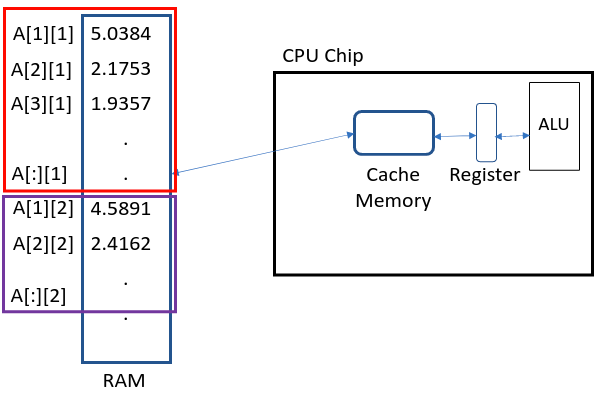
The most important thing to remember is that the data is stored in RAM in a linear fashion (1D).
The first step is to generate a \(5000\times5000\) matrix of random numbers. This is done in Julia as follows:
A = rand(5000, 5000)*10
5000×5000 Matrix{Float64}:
 5.03846   4.58912   7.1005    5.21892   …  4.54396   7.36507   4.01988
 2.17532   2.41624   8.64615   0.84582      2.4431    2.97512   4.40888
 1.93575   0.699285  8.7284    4.6449       1.37964   6.23566   2.98806
 3.83268   8.42017   9.66205   7.14073      7.75752   0.183603  9.57737
 4.6633    2.64513   8.15831   5.45722      8.30875   2.57161   0.02877
 8.80673   2.21542   8.13674   9.93325   …  7.81374   7.65582   8.46948
 7.67453   5.43839   1.6908    8.41406      0.425791  5.46946   8.81717
 1.96266   4.69834   6.08504   2.73894      2.37154   2.1411    2.39905
 0.744606  3.93134   2.12461   1.30628      0.160766  4.52978   9.93005
 9.5532    3.50446   5.16795   0.891007     1.05626   4.37425   2.84276
 9.15744   6.42421   7.94237   1.89686   …  6.61071   9.65093   7.54344
 4.50209   5.50591   8.60566   1.73348      8.66581   5.33027   2.9608
 1.44016   2.79131   9.62346   7.55472      6.54422   4.33858   9.03697
 ⋮                                       ⋱
 5.73005   0.437692  7.03775   5.63305      5.82807   8.73      0.56327
 2.08363   1.23326   5.05221   3.87795      7.64193   5.70619   0.6294
 9.12929   1.17639   9.60084   3.89799   …  6.52743   4.21519   5.92673
 9.35454   6.00617   5.482     9.12613      0.689471  6.18523   6.24744
 4.90895   1.52338   9.34416   7.82992      3.30676   2.2884    5.95591
 1.27204   2.50706   6.54941   3.55047      5.87974   7.33108   5.27113
 3.73647   2.37662   2.22628   4.7821       4.95708   3.00419   4.84946
 6.98472   2.7361    3.44572   3.36757   …  6.0354    9.19172   9.32838
 4.70179   6.49456   0.326857  2.93387      8.12008   2.41638   5.09379
 5.25246   0.102174  5.58784   9.64384      3.47783   9.39589   2.15167
 1.78689   9.9175    3.11802   3.51899      5.82515   0.55363  8.6704
 9.34795   6.2792    0.262552  9.31061      5.51025   9.08796   0.06783
Julia stores this matrix in a column major way, i.e. all elements of column 1 is stored first followed by column 2, 3 and so on.
The next thing we do is go into the functions and execute the code line by line.
Registers
In both functions (colAccess and rowAccess), the first two lines are same
for i in 1:size(A)[1]
	for j in 1:size(A)[2]
When these lines are executed, value of variables i, j, size(A)[1] and size(A)[2] are stored in registers. This is done so that these small values (which are used repeatedly) are stored close to the ALU, hence decreasing the access times.
Access time of a register (time to move data from register to ALU) is negligible hence for programming purposes, it can be considered as 0 clock cycles (atleast relative to RAM).
Next, i and j are used to access the element of the matrix. This is where things get interesting.
Caches
For an instant let’s assume that there’s no cache in between the register and RAM, and we try to access data directly from RAM. When A[j,i] = A[j,i]+1 is executed for i,j=1, element A[1][1] is fetched from the RAM memory locaion 0 and passed to the ALU where 1 is added to it and it’s deposited back to the RAM location it was fetched from. The same thing then happens for A[2][1] followed by A[3][1], A[4][1], and so on. Now the problem with this is that fetching data from RAM is slow (15-100 clock cycles), and to fetch \(5000\times5000\) elements, it’ll take forever (atleast in terms of clock cycles). We can’t use registers to store these values because it’s too small and it already contains CPU instructions and some small constants. To get around this problem, a fast memory called cache is put inside the CPU chip (closer to ALU) which can hold some data for fast accesses. The size of a cache is really small as compared to RAM and can store just a few elements (e.g. RAM on my laptop is 16GB but my i7 CPU has only 9MB of cache).
It’s quite logical to think, why not increase the size of a register? The simple answer to this is cost. Registers are very expensive to make and increasing it’s size will make the CPU super expensive (not to mention the physical size will increase too). Note: The same logic goes for cache memories as well.
In order to understand how caches manage data, a look into the structure of cache is important.
General Structure of Cache Memory
A cache is a hardware managed memory made up of several sets (or lines), which can hold data in a linear fashion.
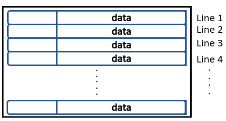
When a data is moved from RAM to a cache line, it’s moved in blocks. Let me illustrate this using the code example.
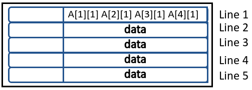
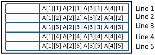
Suppose our cache has 5 lines where each line can hold 4 floating point (64 bit) values. So when the program tries to access A[1][1], the block containing elements [A[1][1],A[2][1],A[3][1],A[4][1]] is moved to the 1st cache line in single go and then required element is fed to ALU from there. The size of this block is decided by the amount a cache line can hold. This is known as Block Size (B).
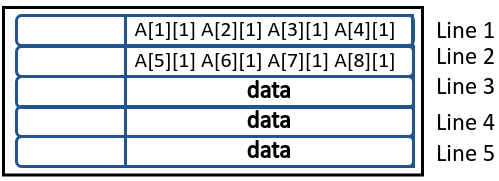
Now in the next iteration when i=2,j=1, element A[2][1] is already in cache so it can be accessed very quickly. Same goes for elements A[3][1] and A[4][1], but when A[5][1] is required, block containing [A[5][1],A[6][1],A[7][1],A[8][1]] is moved to the 2nd cache line in one go, and so on. This solves the problem of slow data accesses from RAM but relies on programmers ability to use Data Locality, i.e. after accessing say A[1][1] it’s programmers responsibility to either reuse A[1][1] or access A[2][1].
When all cache lines are full, eliminations happen where older elements are removed first. For example
[A[21][1],A[22][1],A[23][1],A[24][1]]will be put in cache line 1.
Note that the movement of data in blocks is hardware managed hence it’s super efficient. So we only have to incur a time penalty for the movement of 1st element but following elements can be accessed quickly.
Analysing rowAccess vs colAccess
Let’s now compare the two implementations in detail. For simplicity, I’ll be doing hand simulation of first 6 iterations of both fuctions, but this happens for all other iterations. Also let’s assume it takes 1 clock cycle to fetch data from cache and 50 clock cycles to fetch data from RAM.
- Iteration 1 (
i=1,j=1):- No
A[1][1]in cache so elements[A[1][1],A[2][1],A[3][1],A[4][1]]are placed in cache. colAccesstime: 50 clock cycles.rowAccesstime: 50 clock cycles.
- No
- Iteration 2 (
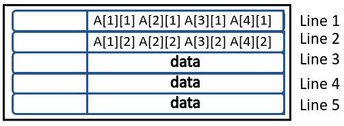
i=i,j=2):colAccesstime: 1 clock cycle asA[2][1]is found in cache. Here’s how cache will look like for this function.
rowAccesstime: 50 clock cycles asA[1][2]is not found in cache. However the whole block will be placed in cache.
I’m considering Fully Associative Cache. Don’t worry, I’ll cover different types of Cache Mappings in another blog.
- Iteration 3 (
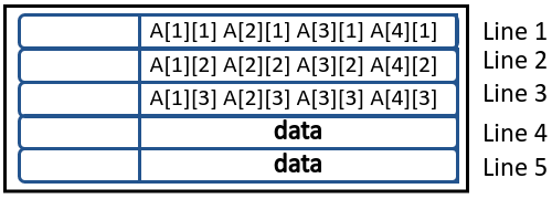
i=i,j=3):colAccesstime: 1 clock cycle asA[3][1]is found in cache. Here’s how cache will look like for this function.
rowAccesstime: 50 clock cycles asA[1][3]is not found in cache. However the whole block will be placed again in cache.
- Iteration 4 (
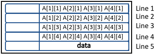
i=i,j=4):colAccesstime: 1 clock cycle asA[4][1]is found in cache. Here’s how cache will look like for this function.
rowAccesstime: 50 clock cycles asA[1][4]is not found in cache. However the whole block will be placed again in cache.
- Iteration 5 (
i=i,j=5):colAccesstime: 50 clock cycles asA[5][1]is not found in cache. Here’s how cache will look like for this function.
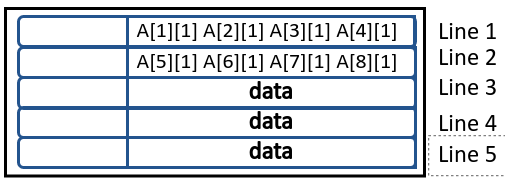
rowAccesstime: 50 clock cycles asA[1][5]is not found in cache. However the whole block will be placed again in cache.
- Iteration 6 (
i=i,j=6):colAccesstime: 1 clock cycle asA[6][1]is found in cache. Here’s how cache will look like for this function.
rowAccesstime: 50 clock cycles asA[1][6]is not found in cache. However the whole block will be placed again in cache after eliminating the data from line 1.
This goes on and on for all the elements and at the end, colAccess will have far fewer cache misses and will run efficiently.
Notice how eliminations are crucial to this. If our matrix was say \(5\times5\), both implementations will be equally efficient.
A = rand(5, 5)*10
5×5 Matrix{Float64}:
2.28675  0.992201  2.73413  0.721498  8.47404
0.40424  8.14012   7.4764   7.52936   3.13966
8.38979  7.98449   9.05752  1.56374   5.53432
8.06838  3.65573   8.05323  4.22322   7.1832
8.04449  3.40892   4.79235  4.87289   1.25914
@btime _ = rowAccess(A); 25.951 ns (0 allocations: 0 bytes)@btime _ = colAccess(A); 23.059 ns (0 allocations: 0 bytes)See how the runtime is almost the same for both now.
Conclusion
This post covers:
- Basics of memory hierarchy of modern computers.
- Movement of data inbetween RAM and Cache.
- Basic workings of Cache.
Useful Links
- Programming Language: Julia Programming Language
- Example Code: jupyter notebook