Finite Differences to evaluate derivatives
Introduction
From Taylor Series expansion we know that
\[f(x+h)=f(x)+hf^{'}(x)+\frac{h^2}{2!}f^{''}(x)+\cdots\]If \(h\) is small enough, we can ignore terms after the first order derivative so that we get
\[f(x+h)\approx f(x)+hf^{'}(x)\]Rearranging the terms, we get a formal definition of calculating derivatives
\[f^{'}(x)\approx \frac{f(x+h)-f(x)}{h}\]Exact derivative is defined as \(f^{'}(x)=\frac{d f}{d x} = \lim_{h\to0} \frac{f(x+h)-f(x)}{h}\)
Claim: The above statement suggests that as \(h \to 0\) (i.e. \(h\) is really small), we can get derivative that is very close to the actual (analytic) derivative.
Let’s try the above claim and see if that holds up in practice. Consider a function \(f(x)=2sin(x)+x^2\).
# Defining Function
f(x::Real) = 2*sin(x) + x^2
Let’s also store the analytical derivative to compare the result against.
# Analytical Derivative
df(x::Real) = 2*cos(x) + 2*x
The plot below shows the error as \(h\) is decreased.
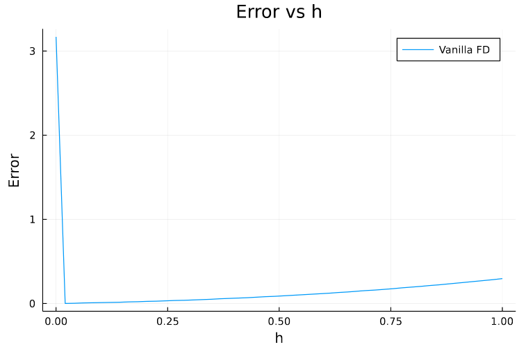
Reason
Let’s see what actually happens in detail. Suppose we choose \(h=10^{-8}\), then \(f(x + h) = 5.818594885328427\) and \(f(x) = 5.818594853651364\).
Notice that \(8^{th}\) digit is the first one that’s different in both, so when these two terms are subtracted we get \(0.0000000316770628\). Next when \(10^{-8}\) is divided, we get \(3.1677062750645733\).
See how only the first few decimal places are relevant and rest are basically junk numbers adding the error. This increases as we further reduce \(h\). For Example, if \(h=10^{-18}\)
\[f(x + h) = 5.818594853651364\] \[f(x) = 5.818594853651364\] \[f(x + h) - f(x) = 0.0\] \[(f(x + h) - f(x)) / h = 0.0\] \[sol = 3.1677063269057153\]
So, the main problem here is due to the fact that we are trying to store the derivative in the same variable (64 bit) as the value which leads to subtraction of two very close numbers (\(f(x+h)\) and \(f(x)\)). This is known as Truncation Error.
What if we could store the derivative in a separate variable?
Complex Step Differentiation
To store the derivative in a separate variable, we can use complex numbers where the real part will define the value of the function and the imaginary part will keep the derivative. This can be written using Taylor Series as follows
\[f(x+\iota h)\approx f(x)+\iota hf^{'}(x)\] \[\iota f^{'}(x) \approx \frac{f(x+\iota h)- f(x)}{h}\] \[f^{'}(x) \approx \text{Imag}\bigg[\frac{f(x+\iota h)- f(x)}{h}\bigg]\] \[f^{'}(x) \approx \text{Imag}\bigg[\frac{f(x+\iota h)}{h}\bigg]\]Let’s solve the same problem as above but using complex numbers now
# Defining Function
f(x::Complex) = 2*sin(x) + x^2
The following function will calcuate the derivate
# Finite DIfference
function complexFiniteDiff(x::Complex)
    df_dx = imag.(f(x))/imag.(x)
    return df_dx
end
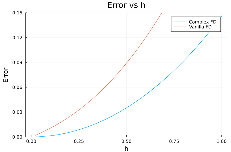
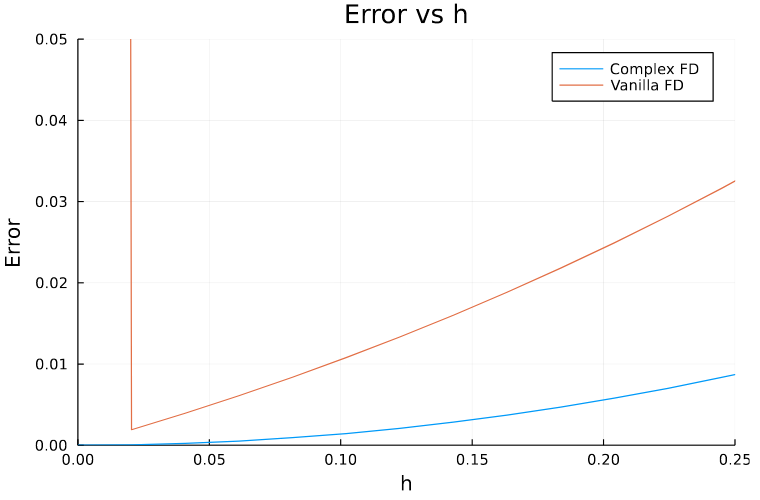
Plotting the results along with the previous case we can see that now the error is not exploding.
Here are the different values in the intermediate steps for \(h=10^{-18}\)
f(complex(x, h)) = 5.818594853651364 + 3.1677063269057185e(-18)im

f(complex(x, 0)) = 5.818594853651364 + 0.0im

f(complex(x, h)) - f(complex(x, 0)) = 0.0 + 3.1677063269057185e(-18)im

imag.(f(complex(x, h))) / h = 3.1677063269057153

sol = 3.1677063269057153
Well, it looks like we’ve solved the problem. Let’s try this method on a more complicated function \(f(x) = \sum_{i=1}^N x \times i\), and see the results for different values of \(N\).
Below are the functions that define the problem.
# Function Definition
function tough(x::Complex)
    f = complex(0,0)
    for i = 1:n
        f += x*i
    end
    return f
end

## Complex Finite Difference
function toughDiff(x::Real, h::Real)
    df = complexFiniteDiff(tough, complex(x,h))
    return df
end

# Analytical Solution
function actualGrad(x::Real)
    df = 0
    for i = 1:n
        df += i
    end
    return df
end
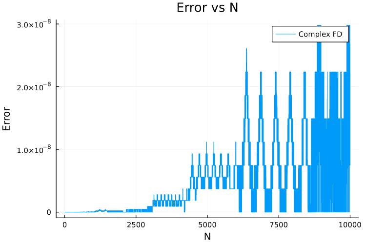
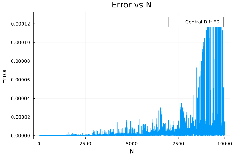
As you can see that errors are quite high for large values of \(N\). This mainly is due to the accumulation of Floating Point errors as the loop is executed inside the function tough.
Is there a way to solve this problem as well? The answer is yes! and Automatic Differentiation is the way to go.
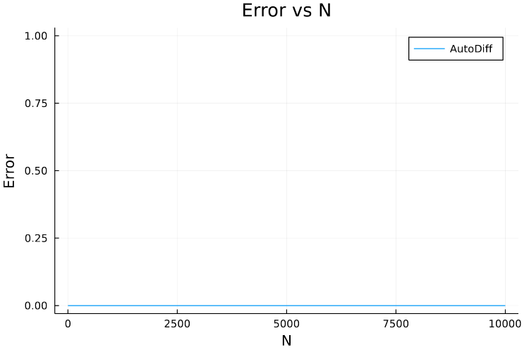
In the next few posts I’ll cover Automatic Differentiation and the two flavours of it (forward and reverse mode AutoDiff).
Conclusion
- In Finite Differences, as the step size decreases, truncation error dominates.
- Truncation Error can be eliminated using the Complex scheme for Finite Differences.
- Roundoff error accumulation in Finite Differences is another problem which makes this method unsuitable for tasks like Deep Learning where thousands of multiplications and additions are performed in long chains.
- This is where Automatic Differentiation comes in handy and is successfully used in several Deep Learning libraries like pytorch.
References
- Programming Language: Julia Programming Language
- Example Code: jupyter notebook
- Awesome Youtube Lecture: Forward-Mode Automatic Differentiation (AD) via High Dimensional Algebras